

Here’s a video I’ve had in mind to do for a year or so, and it’s been some time since I did a polyplot post. And now I’ve finally finished it.
So, a while ago I discovered this polyplot:

It looked pretty neat, but for some time I couldn’t think of a name for it, nor the coloring – eventually (after many custom colormaps), I found one I liked and I thought it fit the ringed structure. Because the colors reminded me of the tropics, I named the structure ‘Tropics’; ‘Tropical Ring’ may also work. This came from like a billion degree 29 polynomials… okay, the exact amount needed to be solved was 1,073,741,824 degree twenty-nine polynomials.

Then, later I discovered another polyplot structure. Its hatching/pattern and shape looked vaguely like the texture and shape of a pineapple to me – so I found some rough pineapple colors and named it ‘Pineapple’. This one also is from degree 29 polynomials.
Pretty neat huh? While both of these structures are quite distinct, fascinating and nothing like each other, what’s more fascinating is that they are related to each other; they’re conjugates.
While any number of polyplots can be made from degree 29 polynomials, these two wildly different polyplots happen to use the same generating coefficients! They are simply close-up views of a much larger structure in the complex plane. The tropics / tropical ring is centered on -i in the complex plane and the pineapple is centered on +i in the complex plane. I wanted to visualize that – how they’re connected. And that’s just what this video shows:
Music is ‘Dream Culture’ by Kevin MacLeod. You may also download the video here: 1080p or 2160p.
I’ve given the overall structure the colorful name of ‘Pineapple Ring’ based on the names of the two smaller structures. I couldn’t say ‘tropical pineapple’ because that’s somewhat redundant as pineapples are already from the tropics.
And now for details of the tedious video construction…
The initial idea was okay – just start at the one spot, zoom out to whole the whole thing, then zoom back in on the other spot. But getting that zoom to look smooth took many attempts. I first tried a few different ways but finally realized I needed something that looked like the error function, but stretched. This led me to skewed normal distributions which I then used the cumulative sum of one of them to control the zoom. Even then, it took multiple attempts fiddling with the parameters to get something I liked.
I told my brother about it and he said I was doing what he called an ‘ease in/out animation’, but that uses Bezier curves whereas I was using a pile of some lesser known statistical math functions for the zooming. He also said I was writing a rendering engine but not using any of the terminology of definitions because I know nothing of animation so all my words are different. I say I wrote a messy Python script hobbled together from spare parts. But I used the cumulative sum of a skewed normal distribution just to zoom a video!
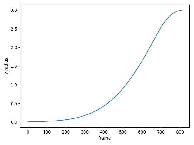
Getting the coloring to look smooth was also a pain. I can’t just set a static limit for all the frames and go with it. The coloring is based on the amount of data in each frame, and that data varies wildly:
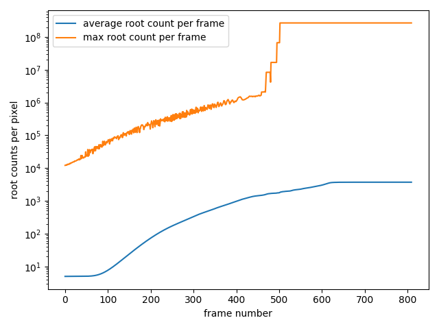
If I set some static cutoff for scaling and trimming the data to color it, the video will look like it’s flickering. And if I base the coloring off of a cutoff point tied to the average of each frame’s data (say +3 or 4 standard deviations from the average), it’ll still look bad as that jumps around too:

So a very tedious manual smoothing was done – first generate the cutoff points for each frame, then Gaussian smooth them out and draw the video frames, then look at it, adjust the cutoff points and smoothing parameters and redraw the frames, take a look again and repeat. There was also some more annoying nonsense to deliberately get that bright flash in the middle of the video. If you watch closely you’ll see the colors still get brighter and dimmer in spots, but its smooth changing and not too noticeable.
After most of the video was done, I then tried to animate the start and end of the video, where it shows the two views, then one spins out or spins in. I wanted to show the two structures, then wanted slide the one out – then decided rotating them in and out, as well as rotating the split view would look cooler. This was a bit easier to do as it was just rotating a static image and cropping, but then I wanted to add multiple colors; so back to redrawing it for every frame! Luckily I saved the underlying data so I didn’t need to spend many hours regenerating them all from scratch; redrawing them would only take ≈2 minutes (this could be sped up more but I didn’t bother writing the code to do that). I ended up using seven different colormaps: Inferno, Laguna, Magma, Plasma, CET L11, Viridis and Tropics (a custom one for Tropics made from 3 colors: #0496b3, #f4a460, #ffd700).
Generating the data for a single frame of this video takes approximately 35 minutes. For the opening and closing frames, I just needed to do that once, then I can plot the image and rotate as needed. But for the body of the video, that’s 1620 unique frames needed. This was done in two segments, 810 frames to zoom out and 810 frames to zoom in. The submodule I previously developed let me generate 810 frames in one shot, and the fancy new computer made it take about 5 hours and 50 minutes while using 25 GB of memory to do so (total working space with all frames and intermediate videos was ≈ 150 GB).
So the information needed for the video could be generated overnight, instead of taking 35 minutes per frame with 1620+ unique frames to do, meaning the whole video would’ve taken ≈ 40 days without that submodule! I suppose I could stretch this out to even more frames making the video slightly longer, but all the manual settings to get the coloring smooth would be defenestrated and I don’t want to spend more tedium doing that! Stitching all the frames into a video however, took just a mere 3 minutes!
All in all, making this video took at least two months to put together (and writing up this post was some additional 12+ hours). All this for a measly 40 second that maybe ten people will ever see! I think I did it mostly because I wanted to see it. Seeing it zoom out and in in my mind and actually seeing it do that for real is pretty satisfying.
And if you like the designs, you can download the ones above to use as computer wallpapers OR purchase them as posters right here:
Note: the posters will look slightly different; they used degree 33 polynomials instead of degree 29 so they’re big enough to print out in 2 foot sizes to hang on the wall! Just like so:

P.S. pineapples taste really terrible, so don’t get me any!

That is really cool! And I love the explanation!